Data Drift¶

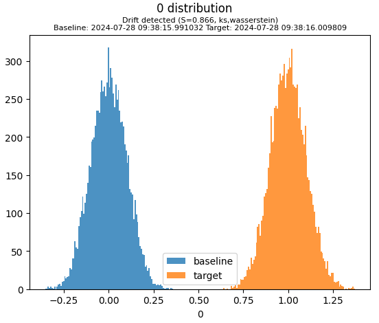
To illustrate data drift monitoring, consider the following example. First we create two datasets, d1 and d2, both a random sample of 1000 points from a normal distribution. We then create a DataDriftMonitor instance and take snapshots of d1 and d2. Finally, we compare the two snapshots and plot the results.

import numpy as np

mu = 0; sigma = 0.1
d1 = np.random.normal(mu, sigma, 10000)
mu = 1; sigma = 0.1
d2 = np.random.normal(mu, sigma, 10000)

from omegaml.backends.monitoring import DataDriftMonitor

with om.runtime.experiment('foo', recreate=True) as exp:
 mon = DataDriftMonitor(tracking=exp)
 mon.snapshot(d1)
 mon.snapshot(d2)

stats = mon.compare()
stats.plot('0')

We can see that the two datasets are similar, as expected, in that they both show a normal distribution. However the second dataset d2 has a different mean and variance than the first dataset d1. This is reflected in the plot.

Understanding drift statistics¶

We can show the data underlying the plot by showing the drift statistics dataframe.

stats.df

The dataframe shows the following information:

column: the column name in the dataset used for the snapshot
statistic: the statistic used to compare the two snapshots
value: the value of the statistic test
pvalue: the p-value of the test
score: the drift score, which is normalized to -1 .. +1 where 0 means no drift and 1 means maximum drift
seq_from: the sequence number of the first snapshot
seq_to: the sequence number of the second snapshot
dt_from: the timestamp of the first snapshot
dt_to: the timestamp of the second snapshot
baseline: the baseline snapshot used for comparison
target: the snapshot used for comparison

The following statistics are computed automatically:

ks: The Kolmogorov-Smirnov statistic (for numeric data)
wasserstein: The Wasserstein distance (for numeric data)
chisq: The Chi-Square statistic (for categorical data)
mean: The mean difference (the mean drift score for all columns)

The sequence number and timestamp are used to track the order of snapshots. Each new call to the monitor.snapshot() method adds a new snapshot, and thus increases the sequence by one. The first snapshot is assigned sequence 0.

Comparing snapshots¶

To compare snapshots, we can specify the specific sequence numbers to compare, either the absolute sequence (0 .. n), where n is the number of snapshots available, or len(monitor), or as a relative negative index. By default the last two snapshots are compared.

# compare the most recent snapshots
stats = mon.compare() # this is equivalent to calling mon.compare(seq=[-2, -1])

If there are more than two snapshots, we can compare any two snapshots by specifying their relative sequence numbers, e.g. to compare the first and last snapshots:

# add a new snapshot
mu = 1; sigma = 0.5
d3 = np.random.normal(mu, sigma, 10000)
mon.snapshot(d3)

# compare the first and last snapshots
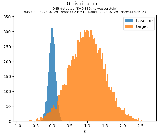
stats = mon.compare(seq=[0, -1])
stats.plot('0')

It is common to have a baseline snapshot that is used for comparison to multiple snapshots taken over time. We can get this comparison by specifying the baseline sequence number or the baseline name. The baseline snapshot is the first snapshot taken, i.e. the one with sequence number 0. We can also specify the baseline by sequence number, using the baseline= kwarg.

# compare all snapshots to the baseline
stats = mon.compare(seq='baseline') # compare all snapshots to the baseline

An alternative to comparing all snapshots to the baseline is to compare all snapshots to their immediate predecessor. This is useful to see how the data drifts over time, assuming that each snapshots represents a new baseline. We can do this by specifying seq=’series’:

# compare all snapshots to their immediate predecessor
stats = mon.compare(seq='series')

Plotting drift over time¶

To plot the drift score over time, we can use the plot() method with kind=’time’:

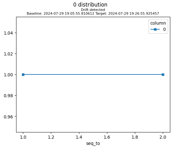
stats.plot('0', kind='time')

This plot shows the drift score between the first snapshot and all subsequent snapshots. The drift score is normalized to -1 .. +1 where 0 means no drift and 1 means maximum drift.

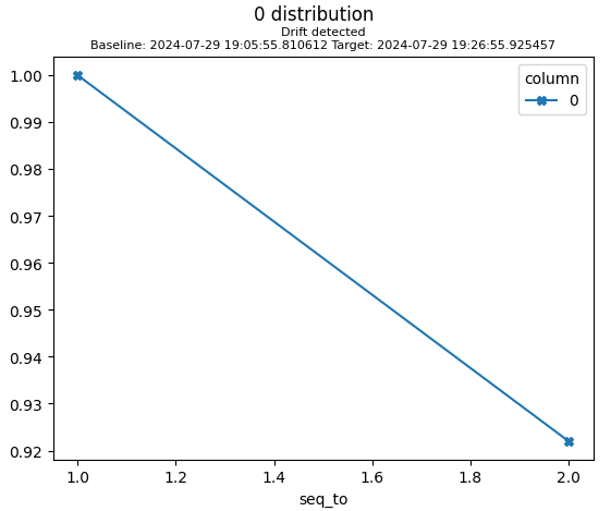
To analyze drift with respect to a specific statistic, specify statistic=<metric>:

stats.plot('0', statistic='ks', kind='time')

To see the statistic’s specific values, we can directly filter the drift statistics dataframe:

stats.df['0', 'ks']